| üāo157.süiS-PlusüjāvāŹāOāēāĆā\ü[āXüä |
| ā_āEāōāŹü[āh |
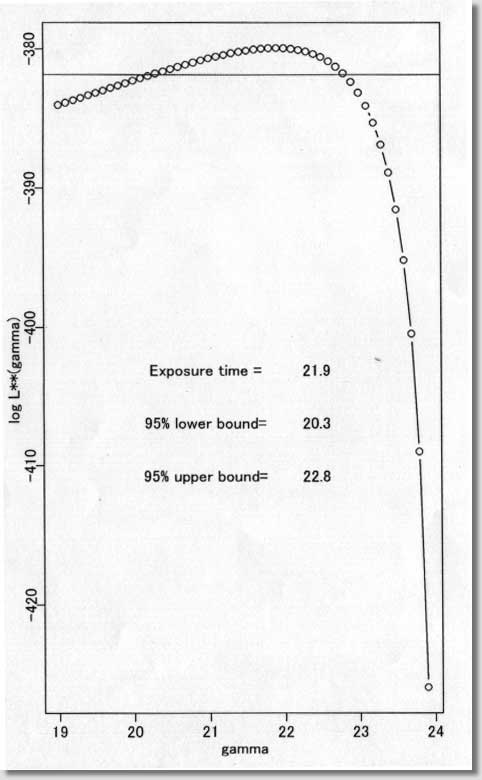
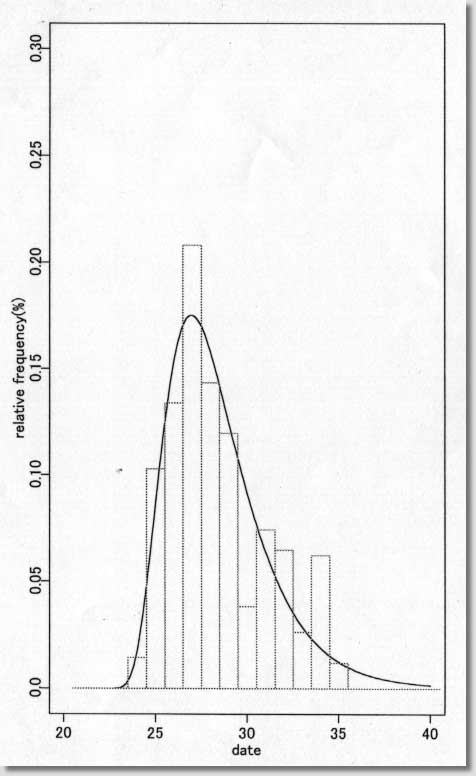
| # Software # Maximum likelihood estimate of date of Infection # under the assumption of lognormal incubation period # ( S-PLUS version 3.2J ) # /s94/o157.s # Programmed by # # T. Tango # Directors of Library and # Division of Theoretical Epidemiology and Biostatistics # Department of Epidemiology # National Institute of Public Health # ----------------------------------------------------------------- # ( README FIRST ) # # 1. This program can be VERY DANGEROUS for NON-LOGNORMAL DISTRIBUTION # for the incubation period. !! # 2. Please read carefully the DISCUSSION SECTION of my paper. # 3. I have no experience of running this program # under S-PLUS version 4 or 5. # 4. You are free to use this software for noncommercial purposes # and even to modify it but please cite this original program. # # Reference: # Tango T. Japanese Journal of Public Health 45, 129-141 (1998). # # ----------------------------------------------------------------- # Input: ts = data vector # sta = starting date # xmin = min of x-axix # xmax = max of x-axis # dens = max of y-axis # hh = width adjustment factor for line search # ----------------- Example ---------------------------------------- # H8 Okayama ken : Figure 1-2 and Table 1 in my paper # Of course, this part depends on your own data. # ts<-c(rep(24,6),rep(25,43),rep(26,56),rep(27,87),rep(28,60),rep(29,50), rep(30,16),rep(31,31),rep(32,27),rep(33,11),rep(34,26), rep(35,5)) sta<-19 xmin<-20 xmax<-40 dens<-0.3 hh<- 10 # -------------------------------------------------------------------- par(mfrow=c(1,2)) jj<-floor(min(ts*hh))-1 st<- sta*hh q<-st:jj ind<-(st:jj)/hh n<-length(ts) for (s in st:jj){ ss<- s/hh; y<-log(ts-ss); m1<-mean(y); v<-var(y) q[s-st+1]<-n*(log(v)+2*m1)*(-1/2) } plot(ind,q,type="b",pch=1,xlab=" gamma ", ylab="log L**(gamma) ") abline(h=max(q)-1.92,col=2) sol<- ind[q==max(q)] pos<-(max(q)+min(q))/2 x1<-st+(jj-st)/5*2 x1<-x1/hh x2<-st+(jj-st)/5*3.5 x2<-x2/hh text(x1,pos, "Exposure time =") text(x2,pos, sol) low95<- min( ind[q>max(q)-1.92] ) upp95<- max( ind[q>max(q)-1.92] ) w<-(max(q)-pos)/6 text(x1,pos-w, "95% lower bound="); text(x2,pos-w,low95) text(x1,pos-w*2,"95% upper bound="); text(x2,pos-w*2,upp95) sk<- sum( (ts-mean(ts))^3 )/(sum( (ts-mean(ts))^2 ))^1.5 * sqrt(n) mu<-mean(log(ts-sol)) sigma<-sqrt( var(log(ts-sol))*(n-1)/n ) linf<- -n/2 * log( var(ts)*(n-1)/n ) lgn<-max(q)-n/2*(1+log(2*3.141593)) soln<- floor(sol*10)+1 # z<-(soln:(xmax*10))/10 plot(z,dlnorm(z-sol,mu,sigma),type="l",xlim=c(xmin,xmax), ylim=c(0,dens), ylab="relative frequency(%)",xlab=" date ") w<-(xmin:xmax)+0.5 h<-1 r<-hist(ts,breaks=w,plot=F) k<-xmax-xmin for (i in 1:k) { a<-c(w[i],w[i],w[i+1],w[i+1],w[i]) b<-c(0,r$count[i],r$count[i],0,0) lines(a,b/n/h,col=5) } # # ------ end ------ |
| ü@ üāāvāŹāOāēāĆÅłŚØīŗē╩āTāōāvāŗüä |
 |
 |

ü@