meet.s（S-Plus）

＜meet.s（S-Plus）プログラムソース＞

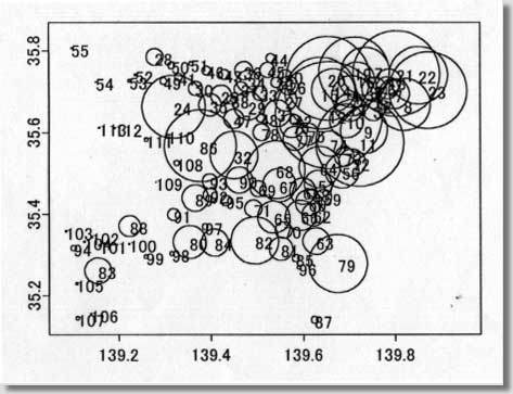
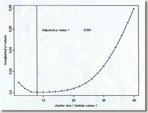
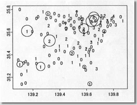
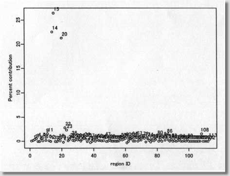
# S-PLUS code for the detection of spatial clustering program
# called MEET (Maximized Excess Events Test)
#
# August 2000 (version 2.00)
#
# Programmed by
#
# Toshiro Tango
# Division of Theoretical Epidemiology
# Department of Epidemiology
# The Institute of Public Health
# 4-6-1 Shirokanedai, Minatoku, Tokyo, 108, Japan
# E-mail: tango@iph.go.jp
#
# ----------------------------------------------------------------
# ( README FIRST )
# 1. Please read my paper carefully before using this program.
# 2. You are free to use this program for noncommercial purposes
# even to modify it but please cite this original program
#
# Reference:
# Tango, T. A test for spatial disease clustering adjusted for
# multiple testing. Statistics in Medicine 19, 191-204 (2000).
# -----------------------------------------------------------------
# INPUT:
#
# nloop: The number of Monte Carlo replications, e.g., 999, 9999.
# us$x: x-value of region centroid, e.g., longitude
# us$y: y-value of region centroid, e.g., latitude
# dc: distance matrix calculated from us$x and us$y
# ( Depending on the user's situation, this should be modified !)
# dat$j: j-th category of the confounders included (j=1,2,...,nk )
# dat$d: observed number of cases
# dat$e: expected number of cases ( or population size)
# kvec: a sequence of lambda values used for the profile p-values
#
# ------------------------------------------------------------------
# Major variables:
#
# nk: the number of strata or categories of all the confounders
# included. For example, if age and sex are the confounders
# included, with 18 different age groups, then there should be
# 18x2 = 36 ( = nk ) categories.
# nr: the number of regions
# nn: the number of cases
# kkk: the number of lambda values
# pxx: sorted p-values due to Monte Carlo replications under
# the null
# ss : per cent contribution to C (equation 14)
# top: region id sorted in the order of the magnitude of ss
# (e.g., top[1] denote the most likely location of cluster,
# if any.)
# pres: The resultant adjusted p-value based on Monte Carlo
# replicates
#
# +++++ An example of execution ++++++++++++++++++++++++++++++++++++
#
# 100 cases: the random sample from clustering model A shown in
# Figure 2 of my paper. The result will be the one
# similar to Figure 3 and 4. The difference will be
# due to Monte Carlo replicates produced.
# These data files are added at the end of email.
#
#
nloop<-999
nk<- 1
kvec<- c(1,2,3,4,5,6,7,8,9,10,11,12,13,14,15,16,17,18,19,20)
kvec<- kvec*2
us <-scan("d:/demo/kanto.geo",list(id=0,x=0,y=0))
dat <-scan("d:/demo/kanto.dat",list(id=0,j=0,d=0,e=0))
#
# These three data files are added at the end of this file.
# It takes about 13 minutes using IBM thinkpad 600E.
#
# ++++++++++++++++++++++++++++++++++++++++++++++++++++++++++++++++++++
par(mfrow=c(1,1))
start<-date()
nr<-length(us$id)
qdat<-rep(0,nr)
p<-rep(0,nr)
w<-matrix(0,nr,nr)
nn<-sum(dat$d)

kkk<- length(kvec)
dc<-matrix(0,nr,nr)
regid<-us$id
frq<-matrix(0,nloop,nr)
pval<-matrix(0,nloop,kkk)
pxx<-rep(0,nloop)
pcc<-pxx

for (i in 1:nr){
for (j in i:nr){
dij<-sqrt(((us$x[i]-us$x[j])*90.15)**2 + # An example
((us$y[i]-us$y[j])*110.9)**2) # for Tokyo area
# dij<-sqrt(((us$x[i]-us$x[j]))**2 +
# ((us$y[i]-us$y[j]))**2)
dc[j,i]<- dij
dc[i,j]<- dij
}
}
#
# Calculation of (1) null distribution of test statistic Pmin
#
for (j in 1:nk){
jdat<- dat$d[dat$j == j]
nj<-sum(jdat)
poo<-dat$e[dat$j == j]
p1<-poo/sum(poo)
pp<-matrix(p1)
w1<-diag(p1)-pp%*%t(pp)
qdat<- qdat + jdat
p<- p+nj*p1
w<- w+nj*w1
py<-p1
vv<-py/sum(py)
cvv<-cumsum(vv)
for (ijk in 1:nloop) {
r1<-hist(runif(nj),breaks=c(0,cvv),plot=F)
frq[ijk,]<- frq[ijk,] + r1$count
}
}
frq<-frq/nn
ori<- qdat
qdat<-qdat/nn
w<- w/nn
p<-p/nn
symbols(us$x,us$y,circles=p,inch=0.50) # Figure 1
text(us$x,us$y,regid,adj= -0.5, col=8)
#
for (k in 1:kkk){
rad<- kvec[k]
ac <- exp( -4 * (dc/rad)^2 )
hh <- ac%*%w
hh2<- hh%*%hh
av <- sum(diag( hh ))
av2<- sum(diag( hh2 ))
av3<- sum(diag( hh2%*%hh ))
skew1<- 2*sqrt(2)*av3/ (av2)^1.5
df1<- 8/skew1/skew1
eg1<-av
vg1<-2*av2
for (ijk in 1:nloop){
q<-frq[ijk,]
gt<-(q-p)%*%ac%*%(q-p)*nn
stat1<-(gt-eg1)/sqrt(vg1)
aprox<-df1+sqrt(2*df1)*stat1
pval[ijk,k]<- 1-pchisq(aprox, df1)
}
}
for (ijk in 1:nloop){
pcc[ijk]<-min( pval[ijk,] )
}
pxx<- sort( pcc )
#
# Calculation of (2) test statistic Pmin and its adjusted p-value
# of observed data
#
ptan<-rep(0,kkk)
gtt<-rep(0,kkk)
jjj<-1:kkk
ep<-p*nn
po<-ppois(ori,ep)
pa<-(po-0.90)/0.10
p1<-ifelse(po > 0.9 & ori>0, pa^3, 0)
symbols(us$x,us$y,circle=p1,inch=0.2) # Figure 2
text(us$x, us$y, ori, col=8)
par(cex=0.5)
par(mar=c(4,3,3,5))
par(mfrow=c(1,2))
par(mgp=c(1.5,0.5,0))
#
for (k in 1:kkk) {
ti<-date()
rad<- kvec[k]
ac <- exp( -4 * (dc/rad)^2 )
hh <- ac%*%w
hh2<- hh%*%hh
av <- sum(diag( hh ))
av2<- sum(diag( hh2 ))
av3<- sum(diag( hh2%*%hh ))
skew1<- 2*sqrt(2)*av3/ (av2)^1.5
df1<- 8/skew1/skew1
eg1<-av
vg1<-2*av2
gt<-(qdat-p)%*%ac%*%(qdat-p)*nn
gtt[k]<-gt
stat1<-(gt-eg1)/sqrt(vg1)
aprox<-df1+sqrt(2*df1)*stat1
ptan[k]<- 1-pchisq(aprox, df1)
}
#
# Figure 3
p22<-min( ptan )
at<-c(pxx,p22)
pres<-length(at[at<=p22])/(length(pxx)+1)
pind<-jjj[ptan==min(ptan)]
plot(kvec,ptan,pch=1,type="b",xlab="cluster size ( lambda values ) ",
ylab=" Unadjusted p-values")
abline(v=kvec[pind])
text((max(kvec)+2*min(kvec))/3,(3*max(ptan)+min(ptan))/4,
"Adjusted p-value = ",col=8)
text((1.5*max(kvec)+min(kvec))/2.5,(3*max(ptan)+min(ptan))/4, pres,col=8)
#
# Figure 4
rad<- kvec[pind]
ac <- exp( -4 * (dc/rad)^2 )
ss<-ac%*%(qdat-p)*nn
ss<-(qdat-p)*ss
ss2<-ss
ss<-ss/sum(ss)*100
plot(regid,ss,pch=1,xlab=" region ID ", ylab=" Percent contribution ")
text(regid+2,ss+1,regid,col=8)
top<-regid[sort.list(-ss)]

end<- date()
#
# End of S-plus file
# ----------------------------------------------------------------
# Below are two data sets for example run
#
# example data : kanto.geo (id, longitude, latitude)
#
1 139.755 35.69056
2 139.7753 35.6675
3 139.7544 35.655
4 139.7075 35.68972
5 139.7564 35.70472
6 139.7844 35.70889
7 139.7989 35.69472
8 139.8197 35.66833
9 139.7333 35.60583
10 139.6956 35.62889
11 139.7236 35.57611
12 139.6564 35.64278
13 139.7014 35.66083
14 139.6669 35.70361
15 139.6397 35.69639
16 139.7186 35.72917
17 139.7369 35.74944
18 139.7867 35.72444
19 139.7122 35.74778
20 139.6553 35.7325
21 139.8036 35.74389
22 139.8508 35.74
23 139.8717 35.70333
24 139.3192 35.66333
25 139.4225 35.69083
26 139.5694 35.71472
27 139.5625 35.68
28 139.2781 35.785
29 139.4808 35.66556
30 139.3667 35.70806
31 139.5442 35.6475
32 139.45 35.54528
33 139.5064 35.69611
34 139.4806 35.72528
35 139.3983 35.66806
36 139.4717 35.75139
37 139.4656 35.70778
38 139.4444 35.68056
39 139.5417 35.7225
40 139.5622 35.73833
41 139.33 35.73556
42 139.5819 35.63167
43 139.4297 35.74222
44 139.5297 35.7825
45 139.5231 35.75306
46 139.3906 35.75167
47 139.4497 35.63389
48 139.5078 35.63472
49 139.2969 35.72611
50 139.3142 35.76417
51 139.3572 35.76889
52 139.2361 35.74139
53 139.2233 35.72667
54 139.1519 35.72361
55 139.0994 35.80639
56 139.6856 35.50556
57 139.6328 35.47389
58 139.6197 35.45056
59 139.6453 35.44139
60 139.6119 35.42833
61 139.5992 35.45667
62 139.6219 35.39917
63 139.6278 35.33417
64 139.6364 35.51583
65 139.5358 35.39306
66 139.5944 35.39722
67 139.5481 35.47139
68 139.5411 35.50917
69 139.5022 35.46306
70 139.5569 35.36139
71 139.4917 35.41444
72 139.7072 35.52639
73 139.6906 35.54056
74 139.6592 35.57306
75 139.6108 35.59639
76 139.5756 35.61694
77 139.5825 35.58611
78 139.5094 35.60083
79 139.6753 35.27889
80 139.3531 35.33222
81 139.5511 35.31528
82 139.4947 35.33583
83 139.1556 35.26139
84 139.4078 35.33056
85 139.5833 35.29222
86 139.3764 35.56806
87 139.6239 35.14083
88 139.2233 35.37139
89 139.3656 35.44
90 139.4611 35.48417
91 139.3183 35.39944
92 139.3986 35.44694
93 139.3975 35.48111
94 139.1031 35.3175
95 139.4325 35.43361
96 139.59 35.26917
97 139.3869 35.36972
98 139.3144 35.30361
99 139.2581 35.29639
100 139.2219 35.3275
101 139.1594 35.32361
102 139.1425 35.345
103 139.0864 35.35917
104 139.1264 35.33306
105 139.1097 35.22944
106 139.1406 35.155
107 139.1114 35.14472
108 139.3247 35.52583
109 139.2797 35.47889
110 139.3061 35.5925
111 139.2594 35.58306
112 139.1922 35.61111
113 139.1586 35.61167
#
# example data: kanto.dat (id, stratum no, number of cases, population)
#
1 1 0 39472
2 1 0 68041
3 1 0 158499
4 1 2 296790
5 1 2 181269
6 1 1 162969
7 1 0 222944
8 1 3 385159
9 1 4 344611
10 1 2 251222
11 1 1 647914
12 1 3 789051
13 1 0 205625
14 1 6 319687
15 1 8 529485
16 1 0 261870
17 1 2 354647
18 1 0 184809
19 1 2 518943
20 1 8 618663
21 1 4 631163
22 1 0 424801
23 1 1 565939
24 1 2 466347
25 1 0 152824
26 1 2 139077
27 1 0 165564
28 1 1 125960
29 1 0 209396
30 1 0 105372
31 1 0 197677
32 1 2 349050
33 1 0 105899
34 1 0 164013
35 1 0 165928
36 1 1 134002
37 1 0 100982
38 1 1 65833
39 1 0 75144
40 1 1 95146
41 1 0 58062
42 1 2 74189
43 1 0 75132
44 1 1 67539
45 1 0 113818
46 1 0 65562
47 1 2 144489
48 1 1 58635
49 1 0 50387
50 1 1 52103
51 1 0 30967
52 1 0 16444
53 1 0 21553
54 1 0 3808
55 1 0 8752
56 1 1 250100
57 1 0 205510
58 1 0 76978
59 1 0 116634
60 1 0 194617
61 1 2 195795
62 1 1 168846
63 1 0 197753
64 1 3 305774
65 1 1 238536
66 1 1 224036
67 1 0 248882
68 1 2 426663
69 1 0 119575
70 1 0 123766
71 1 2 126866
72 1 0 200056
73 1 1 142320
74 1 0 187707
75 1 0 165081
76 1 0 175570
77 1 2 177742
78 1 0 125127
79 1 3 433358
80 1 0 245950
81 1 1 174307
82 1 1 350330
83 1 1 193417
84 1 0 201675
85 1 1 56704
86 1 1 531542
87 1 1 52440
88 1 1 155620
89 1 0 197283
90 1 1 194866
91 1 0 89567
92 1 1 105822
93 1 1 112102
94 1 1 42600
95 1 0 77926
96 1 0 29536
97 1 0 44532
98 1 0 31599
99 1 1 29415
100 1 0 10054
101 1 0 14895
102 1 0 13097
103 1 0 14342
104 1 0 11941
105 1 0 19365
106 1 0 9588
107 1 0 27717
108 1 2 40424
109 1 0 3549
110 1 0 21535
111 1 0 28038
112 1 0 10592
113 1 1 10729
# -------------- End of all files ----------------------

　
＜プログラム処理結果サンプル＞