| üārefcurve.süiS-PlusüjāvāŹāOāēāĆā\ü[āXüä | |
| refcurve1.s | ā_āEāōāŹü[āh |
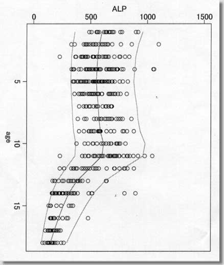
| # S-PLUS program arrl.prg (No. 1 : Estimation
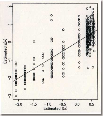
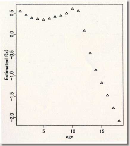
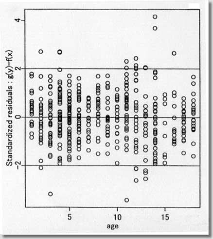
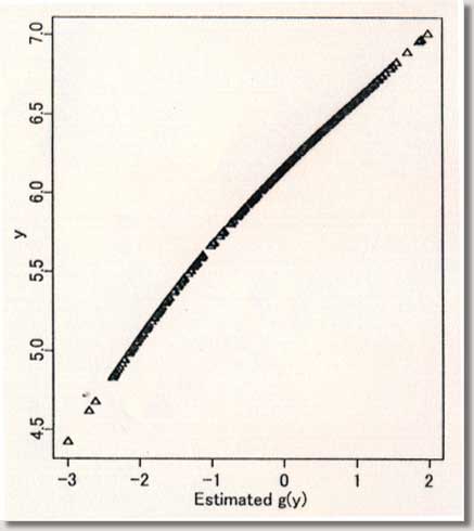
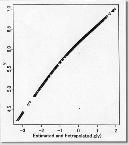
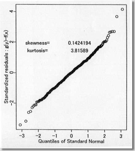
procedures ) September 1996 # Programmed by # # Toshiro Tango # Division of Theoretical Epidemiology # Department of Epidemiology # The Institute of Public Health # 4-6-1 Shirokanedai, Minatoku, Tokyo, 108, Japan # E-mail: tango@iph.go.jp # # +++++ Program for age-specific reference ranges via smoother AVAS # +++++ This program uses log-transformed y-value # +++++ and exponentiates the results. # +++++ # +++++ DATA vectors (ddx,ddy) # # ddx <- x-value vector (ex. age) # ddy <- y-value vector (ex. foot length) # # +++++ THREE IMPORTANT PARAMETERS : (spanvar,cutm,cuth) # # cuth <- 1.5 : default setting # lower limit of data for upper tail extrapolation # cutm <- -1.5 : default setting # upper limit of data for lower tail extrapolation # spanvar <- 100 : default setting (= Cross Validatin method) # span value for variance function smoother # User specified span value # should be within the range [0, 1) # # +++++ FOUR Parameters necessary for plotting data # # yname<- label of Y variable # xname<- label of Y variable # yup <- upper limit of Y-axis # ylow <- lower limit of Y-axis # # +++++ An example of execution # Data on 450 measurments of foot length and gestatinal age # ( see Altman(1993, Stat. in Med., 12, p917-924) # # ddx<- foot.age ; ddy<- foot ; cuth<- 1.5; cutm<- -1.5; spanvar<-100 # xname<-" gestational age (weeks)"; yname<-" Foot length (mm) " # yup<-100 ; ylow<- 0 # source("arrl.prg1") # par(cex=0.5) par(mar=c(4,3,0.5,0.5)) par(mfrow=c(2,3)) par(mgp=c(1.5,0.5,0)) ddx<-scan("d:/demo/alpage.dat")/360 ddy<-scan("d:/demo/alp.dat") cuth<-1.5 cutm<- -1.5 spanvar<- 100 xname<- " age " yname<- " ALP " yup<- 1500 ylow<- 0 # x <- ddx yval <- ddy # if (min(yval) == 0 ){ cons<-1 } else { cons<-0 } # this part should be yval<-log(yval+cons) # deleted when untransformed # y-values are used # if (spanvar<=1 ){ a<-avas(x,yval,span.var=spanvar) } else { a<-avas(x,yval) } plot(x,a$tx,pch=2,ylab="Estimated f(x)",xlab=xname) flag<-0 hflag<-0 lflag<-0 nn<-length(x) # plot(a$ty,yval,pch=2,xlab=" Estimated g(y)",ylab=" y") sdev<-sqrt(var(a$ty-a$tx)) m<-approx(a$ty,yval,a$tx) if ( max(a$tx+1.96*sdev) <= max(a$ty) ){ h<-approx(a$ty,yval,a$tx+1.96*sdev) } else { # fit<-lsfit(a$ty[a$ty > cuth],yval[a$ty > cuth]) aty<-a$ty[a$ty > cuth] fit<-lm(yval[a$ty > cuth] ~ aty+aty^2 ) deltax<-seq(max(a$ty),max(a$tx+2.10*sdev),by=0.02) deltay<-fit$coef[1]+fit$coef[2]*deltax+fit$coef[3]*deltax^2 h<-approx(c(a$ty,deltax),c(yval,deltay),a$tx+1.96*sdev) flag<-1 hflag<-1} if ( min(a$tx-1.96*sdev) >= min(a$ty) ){ lx<-approx(a$ty,yval,a$tx-1.96*sdev) } else { # fit<-lsfit(a$ty[a$ty < cutm],yval[a$ty < cutm]) aty<-a$ty[a$ty < cutm] fit<-lm(yval[a$ty < cutm] ~ aty+aty^2 ) deltax2<-seq(min(a$tx-2.10*sdev), min(a$ty),by=0.02) deltay2<-fit$coef[1]+fit$coef[2]*deltax2+fit$coef[3]*deltax2^2 lx<-approx(c(deltax2,a$ty),c(deltay2,yval),a$tx-1.96*sdev) flag<-1 lflag<-1} if (hflag==1 & lflag==0) { plot(c(a$ty,deltax),c(yval,deltay),pch=2, xlab=" Estimated and Extrapolated g(y)", ylab= "y") } if (hflag==0 & lflag==1) { plot(c(deltax2,a$ty),c(deltay2,yval),pch=2, xlab=" Estimated and Extrapolated g(y)", ylab=" y" ) } if (hflag==1 & lflag==1) { plot(c(deltax2,a$ty,deltax),c(deltay2,yval,deltay),pch=2, xlab=" Estimated and Extrapolated g(y)", ylab=" y" ) } plot(a$tx,a$ty,pch=1, xlab="Estimated f(x)", ylab="Estimated g(y)") abline(0,1) xs<-sort(x) mea<-m$y[sort.list(x)] upp<-h$y[sort.list(x)] lowx<-lx$y[sort.list(x)] plot(x,(a$ty-a$tx)/sdev,pch=1, xlab=xname, ylab="Standardized residuals : g(y)-f(x)") abline(h=c(-2,0,2)) tt<-(a$ty-a$tx)/sdev qqnorm(tt,ylab="Standardized residuals : g(y)-f(x)") skew <- sqrt(nn)*sum(tt^3)/(sum(tt^2))^1.5 kurt <- nn*sum(tt^4)/(sum(tt^2))^2 text(-2,2,"skewness= ") text( 0.5,2,skew) text(-2,1.5,"kurtosis= ") text( 0.5,1.5,kurt) # # end of program No.1 # par(mfrow=c(1,2)) # plot(x,exp(yval)-cons,ylim=c(ylow,yup),xlab=xname,ylab=yname,pch=1) #: 4 |
|
| refcurve2.s | ā_āEāōāŹü[āh |
| # program arrl.prg (No.2: final plots) # # par(mfrow=c(1,1)) par(mar=c(7,10,7,10)) nage<-length(unique(xs)) avasmat<-matrix(0,nage,4) avasmat[,1]<-unique(xs) avasmat[,2]<-unique(exp(lowx)-cons) # :1 avasmat[,3]<-unique(exp(mea)-cons) # :2 avasmat[,4]<-unique(exp(upp)-cons) # ;3 # plot(x,exp(yval)-cons,ylim=c(ylow,yup),xlab=xname,ylab=yname,pch=1) #: 4 plot(x,exp(yval)-cons,ylim=c(ylow,yup),xlab=xname,ylab=yname,pch=1) #: 4 # # ++++ When untransformed data are used, the above parts 1-4 should be # ++++ replaced by the following parts 1-4. # # avasmat[,2]<-unique(lowx) # :1 # avasmat[,3]<-unique(mea) # :2 # avasmat[,4]<-unique(upp) # :3 # plot(x,yval,ylim=c(ylow,yup),xlab=xname,ylab=yname,pch=1) # :4 # lines(avasmat[,1],avasmat[,2],col=5) lines(avasmat[,1],avasmat[,3],col=18) lines(avasmat[,1],avasmat[,4],col=5) # # end of program No.2 |
|
| ü@ üāāvāŹāOāēāĆÅłŚØīŗē╩āTāōāvāŗüä |
|
 |
|
 |
|
 |
|
 |
|
 |
|
 |
|
 |
|

ü@